Crash Sequence of Events
Source:vignettes/Crash_sequence_of_events.Rmd
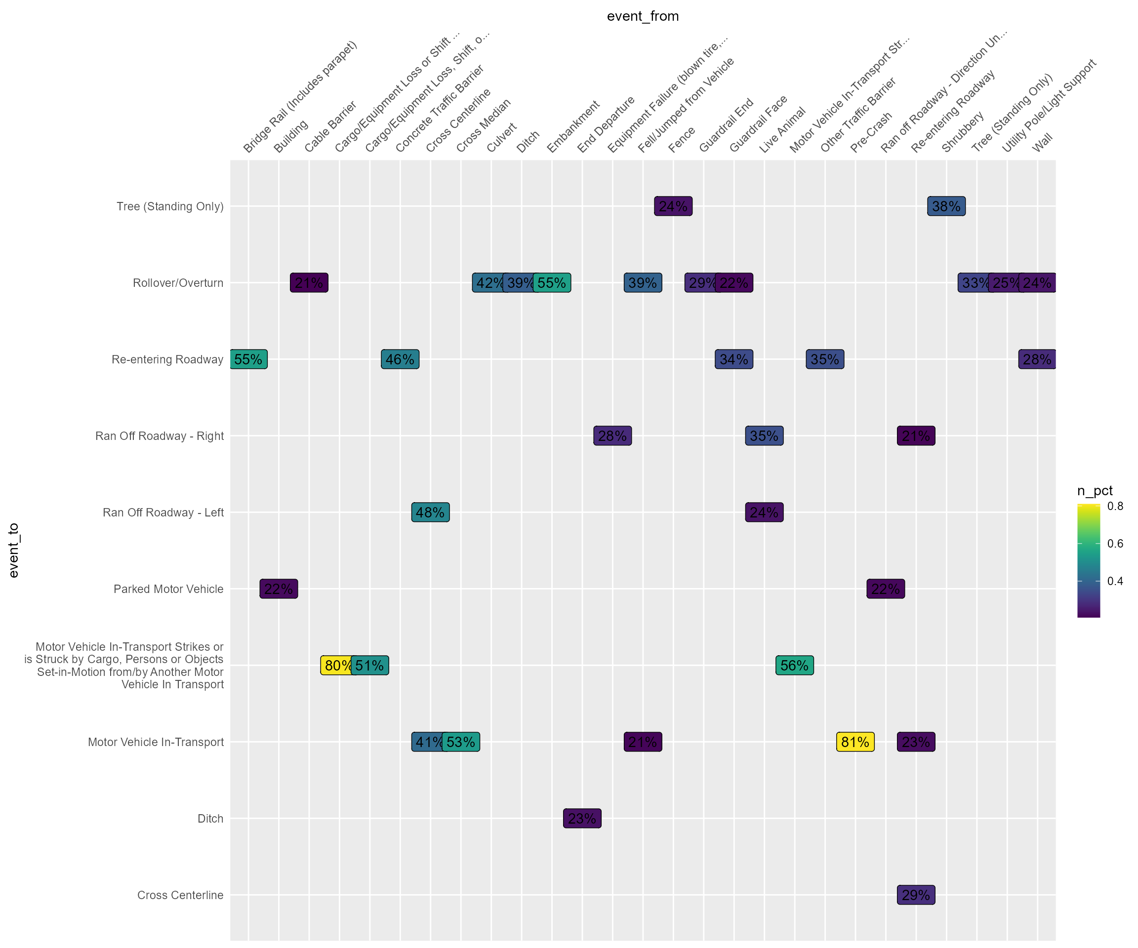
Crash_sequence_of_events.RmdThis vignette explores the vsoe (Vehicle Sequence of Events) data to visualize crash sequence patterns.
vsoe is one of three event-based data files, the
others being cevent and vevent.
According to the CRSS
Analytical User’s Manual, vevent “has the same data
elements as the cevent data file” plus “a data element
that records the sequential event number for each vehicle,” and the
vsoe file “has a subset of the data elements contained
in the Vevent data file (it is a simplified
vevent data file)” (p. 16). rfars
therefore omits cevent and vevent.
For this analysis, we will use one year of data from CRSS and explore which crash events were associated with more severe crash outcomes.
mydata <- rfars::get_gescrss(years=2023, proceed = TRUE)
my_events <- mydata$events
Below is the sequence for one randomly selected crash:
| casenum | veh_no | aoi | soe | veventnum | year |
|---|---|---|---|---|---|
| 202304741191 | 1 | 12 Clock Point | Motor Vehicle In-Transport | 1 | 2023 |
| 202304741191 | 2 | Left-Back Side | Motor Vehicle In-Transport | 1 | 2023 |
| 202304741191 | 2 | Non-Harmful Event | Ran Off Roadway - Right | 2 | 2023 |
| 202304741191 | 2 | Non-Harmful Event | Re-entering Roadway | 3 | 2023 |
| 202304741191 | 2 | Non-Collision | Rollover/Overturn | 4 | 2023 |
| 202304741191 | 2 | Non-Harmful Event | Ran Off Roadway - Left | 5 | 2023 |
| 202304741191 | 2 | Right-Back Side | Ditch | 6 | 2023 |
After some moderate data wrangling, the event sequences can be compared by severity across regions, as shown below. This figure shows how many fatal and non-fatal crashes occurred in 2023 by region. It filters to event sequences that end with “Pedestrian” and shows the preceding events in order. The most common crash sequence begins and ends with “Pedestrian.” The top-left panel of the graph indicates that 37 fatal pedestrian crashes in the midwest were preceded by a vehicle running off the roadway in an unknown direction. The other 516-31= were single-event crashes beginning and ending with striking the pedestrian. Fatal pedestrian crashes in the northeast followed 4 distinct patterns, including the single-event sequence; 5 patterns emerge in the south; etc. With the exception of the midwest, all other crash sequences involved running off the roadway to the right. Notably, running off the roadway to the left was much more common among non-fatal crashes.
events_temp <-
  my_events %>%
  group_by(casenum, veh_no) %>%
  mutate(
    veventnum = as.numeric(as.character(veventnum)),
    lasteventnum = max(veventnum)
  ) %>%
  ungroup() %>%
  filter(soe=="Pedestrian" & veventnum==lasteventnum) %>%
  distinct(casenum, veh_no, year, lasteventnum) %>%
  left_join(events_data$events) %>%
  left_join(
    distinct(events_data$flat, year, region, casenum, max_sev, weight) %>%
      mutate_at(c("casenum", "year"), as.character) %>%
      mutate_at(c("region"), word)
  ) %>%
  mutate(
    fatal = factor(ifelse(max_sev != "Fatal Injury (K)", "Non-Fatal", "Fatal"), ordered = T),
    veventnum = as.numeric(as.character(veventnum)),
    eventnum = as.factor(veventnum - lasteventnum),
    soe = str_replace_all(soe, "Motor Vehicle In-Transport Strikes or is Struck by Cargo, Persons or Objects Set-in-Motion from/by Another Motor Vehicle In Transport", "Motor Vehicle In-Transport Strikes or is Struck by Something")
  )

sequences <-
  events_temp %>%
  arrange(casenum, eventnum) %>%
  distinct(casenum, region, eventnum, soe, fatal) %>%
  group_by(casenum, region, fatal) %>%
  summarize(sequence = paste0(soe, collapse = " THEN "), .groups = "drop")

sequences_meta <-
  sequences %>%
  group_by(sequence, region, fatal) %>%
  summarize(sequence_n = n(), .groups = "drop") %>%
  arrange(-sequence_n) %>%
  mutate(sequence_num = row_number()) %>%
  filter(sequence_n > 1)

sequence_event_counts <-
  inner_join(events_temp, sequences) %>%
  group_by(sequence, soe, eventnum, region, fatal) %>%
  summarize(n=sum(weight)) %>%
  filter(sequence %in% unique(sequences_meta$sequence))

event_counts <-
  sequence_event_counts %>%
  group_by(soe, eventnum, region, fatal) %>%
  summarize(n=sum(n))

sequence_event_counts %>%
  ggplot(aes(x=eventnum, y=soe, group=sequence)) +
  geom_line(aes(linewidth = log(n)), alpha=.6) +
  geom_label(
    inherit.aes = F,
    data = event_counts,
    aes(x=eventnum, y=soe, size=log(n), label = scales::comma(n, accuracy = 1))
  ) +
  scale_x_discrete(expand = expansion(add=c(.2, .6))) +
  facet_grid(fatal~region, scales = "free_y", space = "free_y") +
  guides(size="none", linewidth="none") +
  labs(
    x = "Event Number (Relative to Last Event)",
    y = NULL,
    title = "Crash Sequences",
    subtitle = "Pedestrian crashes in 2023"
  ) +
  theme(
    axis.ticks = element_blank(),
    strip.text.y.right = element_text(angle=0)
  )
This topic could be explored further with other data elements and techniques. The event sequence data represents an underused resource for this research.