A first step in many transportation safety analyses involves counting
the number of relevant crashes, fatalities, or people involved.
counts() lets users specify what to count,
where to count them (rural/urban and/or in specified states or
regions), who to include, the interval over which to
count (annually or monthly), and factors involved in the
crashes. It returns a simple tibble that can be easily piped into
ggplot() to quickly visualize counts.
First we load the required libraries:
annual_counts
rfars includes annual_counts, a table of
annual crash counts:
knitr::kable(rfars::annual_counts, format = "html")| year | what | states | region | urb | who | involved | n | source |
|---|---|---|---|---|---|---|---|---|
| 2015 | crashes | all | all | all | all | any | 32538.00 | FARS |
| 2016 | crashes | all | all | all | all | any | 34748.00 | FARS |
| 2017 | crashes | all | all | all | all | any | 34560.00 | FARS |
| 2018 | crashes | all | all | all | all | any | 33919.00 | FARS |
| 2019 | crashes | all | all | all | all | any | 33487.00 | FARS |
| 2020 | crashes | all | all | all | all | any | 35935.00 | FARS |
| 2021 | crashes | all | all | all | all | any | 39785.00 | FARS |
| 2022 | crashes | all | all | all | all | any | 39422.00 | FARS |
| 2023 | crashes | all | all | all | all | any | 37654.00 | FARS |
| 2015 | crashes | all | all | all | all | alcohol | 9215.00 | FARS |
| 2015 | crashes | all | all | all | all | bicyclist | 831.00 | FARS |
| 2015 | crashes | all | all | all | all | distracted driver | 3619.00 | FARS |
| 2015 | crashes | all | all | all | all | drugs | 3058.00 | FARS |
| 2015 | crashes | all | all | all | all | hit and run | 1761.00 | FARS |
| 2015 | crashes | all | all | all | all | large trucks | 3583.00 | FARS |
| 2015 | crashes | all | all | all | all | motorcycle | 4942.00 | FARS |
| 2015 | crashes | all | all | all | all | older driver | 6109.00 | FARS |
| 2015 | crashes | all | all | all | all | pedalcyclist | 831.00 | FARS |
| 2015 | crashes | all | all | all | all | pedbike | 6294.00 | FARS |
| 2015 | crashes | all | all | all | all | pedestrian | 5466.00 | FARS |
| 2015 | crashes | all | all | all | all | police pursuit | 311.00 | FARS |
| 2015 | crashes | all | all | all | all | roadway departure | 16970.00 | FARS |
| 2015 | crashes | all | all | all | all | rollover | 7854.00 | FARS |
| 2015 | crashes | all | all | all | all | speeding | 8706.00 | FARS |
| 2015 | crashes | all | all | all | all | young driver | 4195.00 | FARS |
| 2016 | crashes | all | all | all | all | alcohol | 9308.00 | FARS |
| 2016 | crashes | all | all | all | all | bicyclist | 848.00 | FARS |
| 2016 | crashes | all | all | all | all | distracted driver | 3512.00 | FARS |
| 2016 | crashes | all | all | all | all | drugs | 3512.00 | FARS |
| 2016 | crashes | all | all | all | all | hit and run | 2012.00 | FARS |
| 2016 | crashes | all | all | all | all | large trucks | 4134.00 | FARS |
| 2016 | crashes | all | all | all | all | motorcycle | 5255.00 | FARS |
| 2016 | crashes | all | all | all | all | older driver | 6701.00 | FARS |
| 2016 | crashes | all | all | all | all | pedalcyclist | 853.00 | FARS |
| 2016 | crashes | all | all | all | all | pedbike | 6897.00 | FARS |
| 2016 | crashes | all | all | all | all | pedestrian | 6054.00 | FARS |
| 2016 | crashes | all | all | all | all | police pursuit | 358.00 | FARS |
| 2016 | crashes | all | all | all | all | roadway departure | 17936.00 | FARS |
| 2016 | crashes | all | all | all | all | rollover | 8265.00 | FARS |
| 2016 | crashes | all | all | all | all | speeding | 9262.00 | FARS |
| 2016 | crashes | all | all | all | all | young driver | 4412.00 | FARS |
| 2017 | crashes | all | all | all | all | alcohol | 9296.00 | FARS |
| 2017 | crashes | all | all | all | all | bicyclist | 805.00 | FARS |
| 2017 | crashes | all | all | all | all | distracted driver | 3368.00 | FARS |
| 2017 | crashes | all | all | all | all | drugs | 3701.00 | FARS |
| 2017 | crashes | all | all | all | all | hit and run | 1956.00 | FARS |
| 2017 | crashes | all | all | all | all | large trucks | 4325.00 | FARS |
| 2017 | crashes | all | all | all | all | motorcycle | 5159.00 | FARS |
| 2017 | crashes | all | all | all | all | older driver | 6774.00 | FARS |
| 2017 | crashes | all | all | all | all | pedalcyclist | 811.00 | FARS |
| 2017 | crashes | all | all | all | all | pedbike | 6842.00 | FARS |
| 2017 | crashes | all | all | all | all | pedestrian | 6039.00 | FARS |
| 2017 | crashes | all | all | all | all | police pursuit | 367.00 | FARS |
| 2017 | crashes | all | all | all | all | roadway departure | 17397.00 | FARS |
| 2017 | crashes | all | all | all | all | rollover | 7986.00 | FARS |
| 2017 | crashes | all | all | all | all | speeding | 8955.00 | FARS |
| 2017 | crashes | all | all | all | all | young driver | 4256.00 | FARS |
| 2018 | crashes | all | all | all | all | alcohol | 8708.00 | FARS |
| 2018 | crashes | all | all | all | all | bicyclist | 873.00 | FARS |
| 2018 | crashes | all | all | all | all | distracted driver | 2643.00 | FARS |
| 2018 | crashes | all | all | all | all | drugs | 3780.00 | FARS |
| 2018 | crashes | all | all | all | all | hit and run | 1995.00 | FARS |
| 2018 | crashes | all | all | all | all | large trucks | 4404.00 | FARS |
| 2018 | crashes | all | all | all | all | motorcycle | 4953.00 | FARS |
| 2018 | crashes | all | all | all | all | older driver | 6831.00 | FARS |
| 2018 | crashes | all | all | all | all | pedalcyclist | 876.00 | FARS |
| 2018 | crashes | all | all | all | all | pedbike | 7207.00 | FARS |
| 2018 | crashes | all | all | all | all | pedestrian | 6339.00 | FARS |
| 2018 | crashes | all | all | all | all | police pursuit | 358.00 | FARS |
| 2018 | crashes | all | all | all | all | roadway departure | 16844.00 | FARS |
| 2018 | crashes | all | all | all | all | rollover | 7393.00 | FARS |
| 2018 | crashes | all | all | all | all | speeding | 8632.00 | FARS |
| 2018 | crashes | all | all | all | all | young driver | 4032.00 | FARS |
| 2019 | crashes | all | all | all | all | alcohol | 8647.00 | FARS |
| 2019 | crashes | all | all | all | all | bicyclist | 859.00 | FARS |
| 2019 | crashes | all | all | all | all | distracted driver | 2872.00 | FARS |
| 2019 | crashes | all | all | all | all | drugs | 3858.00 | FARS |
| 2019 | crashes | all | all | all | all | hit and run | 1969.00 | FARS |
| 2019 | crashes | all | all | all | all | large trucks | 4460.00 | FARS |
| 2019 | crashes | all | all | all | all | motorcycle | 4943.00 | FARS |
| 2019 | crashes | all | all | all | all | older driver | 7101.00 | FARS |
| 2019 | crashes | all | all | all | all | pedalcyclist | 862.00 | FARS |
| 2019 | crashes | all | all | all | all | pedbike | 7107.00 | FARS |
| 2019 | crashes | all | all | all | all | pedestrian | 6251.00 | FARS |
| 2019 | crashes | all | all | all | all | police pursuit | 359.00 | FARS |
| 2019 | crashes | all | all | all | all | roadway departure | 16317.00 | FARS |
| 2019 | crashes | all | all | all | all | rollover | 7197.00 | FARS |
| 2019 | crashes | all | all | all | all | speeding | 8650.00 | FARS |
| 2019 | crashes | all | all | all | all | young driver | 3863.00 | FARS |
| 2020 | crashes | all | all | all | all | alcohol | 9586.00 | FARS |
| 2020 | crashes | all | all | all | all | bicyclist | 945.00 | FARS |
| 2020 | crashes | all | all | all | all | distracted driver | 2885.00 | FARS |
| 2020 | crashes | all | all | all | all | drugs | 5006.00 | FARS |
| 2020 | crashes | all | all | all | all | hit and run | 2519.00 | FARS |
| 2020 | crashes | all | all | all | all | large trucks | 4417.00 | FARS |
| 2020 | crashes | all | all | all | all | motorcycle | 5540.00 | FARS |
| 2020 | crashes | all | all | all | all | older driver | 6517.00 | FARS |
| 2020 | crashes | all | all | all | all | pedalcyclist | 951.00 | FARS |
| 2020 | crashes | all | all | all | all | pedbike | 7481.00 | FARS |
| 2020 | crashes | all | all | all | all | pedestrian | 6538.00 | FARS |
| 2020 | crashes | all | all | all | all | police pursuit | 462.00 | FARS |
| 2020 | crashes | all | all | all | all | roadway departure | 17994.00 | FARS |
| 2020 | crashes | all | all | all | all | rollover | 8149.00 | FARS |
| 2020 | crashes | all | all | all | all | speeding | 10286.00 | FARS |
| 2020 | crashes | all | all | all | all | young driver | 4430.00 | FARS |
| 2021 | crashes | all | all | all | all | alcohol | 10458.00 | FARS |
| 2021 | crashes | all | all | all | all | bicyclist | 973.00 | FARS |
| 2021 | crashes | all | all | all | all | distracted driver | 3211.00 | FARS |
| 2021 | crashes | all | all | all | all | drugs | 5431.00 | FARS |
| 2021 | crashes | all | all | all | all | hit and run | 2829.00 | FARS |
| 2021 | crashes | all | all | all | all | large trucks | 5188.00 | FARS |
| 2021 | crashes | all | all | all | all | motorcycle | 6073.00 | FARS |
| 2021 | crashes | all | all | all | all | older driver | 7515.00 | FARS |
| 2021 | crashes | all | all | all | all | pedalcyclist | 978.00 | FARS |
| 2021 | crashes | all | all | all | all | pedbike | 8395.00 | FARS |
| 2021 | crashes | all | all | all | all | pedestrian | 7424.00 | FARS |
| 2021 | crashes | all | all | all | all | police pursuit | 439.00 | FARS |
| 2021 | crashes | all | all | all | all | roadway departure | 19282.00 | FARS |
| 2021 | crashes | all | all | all | all | rollover | 8826.00 | FARS |
| 2021 | crashes | all | all | all | all | speeding | 11218.00 | FARS |
| 2021 | crashes | all | all | all | all | young driver | 4970.00 | FARS |
| 2022 | crashes | all | all | all | all | alcohol | 10318.00 | FARS |
| 2022 | crashes | all | all | all | all | bicyclist | 1097.00 | FARS |
| 2022 | crashes | all | all | all | all | distracted driver | 3054.00 | FARS |
| 2022 | crashes | all | all | all | all | drugs | 4915.00 | FARS |
| 2022 | crashes | all | all | all | all | hit and run | 2895.00 | FARS |
| 2022 | crashes | all | all | all | all | large trucks | 5298.00 | FARS |
| 2022 | crashes | all | all | all | all | motorcycle | 6192.00 | FARS |
| 2022 | crashes | all | all | all | all | older driver | 7905.00 | FARS |
| 2022 | crashes | all | all | all | all | pedalcyclist | 1097.00 | FARS |
| 2022 | crashes | all | all | all | all | pedbike | 8636.00 | FARS |
| 2022 | crashes | all | all | all | all | pedestrian | 7545.00 | FARS |
| 2022 | crashes | all | all | all | all | police pursuit | 490.00 | FARS |
| 2022 | crashes | all | all | all | all | roadway departure | 18725.00 | FARS |
| 2022 | crashes | all | all | all | all | rollover | 14490.00 | FARS |
| 2022 | crashes | all | all | all | all | speeding | 10934.00 | FARS |
| 2022 | crashes | all | all | all | all | young driver | 4719.00 | FARS |
| 2023 | crashes | all | all | all | all | alcohol | 9324.00 | FARS |
| 2023 | crashes | all | all | all | all | bicyclist | 1155.00 | FARS |
| 2023 | crashes | all | all | all | all | distracted driver | 3021.00 | FARS |
| 2023 | crashes | all | all | all | all | drugs | 4167.00 | FARS |
| 2023 | crashes | all | all | all | all | hit and run | 2783.00 | FARS |
| 2023 | crashes | all | all | all | all | large trucks | 4925.00 | FARS |
| 2023 | crashes | all | all | all | all | motorcycle | 6241.00 | FARS |
| 2023 | crashes | all | all | all | all | older driver | 7807.00 | FARS |
| 2023 | crashes | all | all | all | all | pedalcyclist | 1155.00 | FARS |
| 2023 | crashes | all | all | all | all | pedbike | 8427.00 | FARS |
| 2023 | crashes | all | all | all | all | pedestrian | 7277.00 | FARS |
| 2023 | crashes | all | all | all | all | police pursuit | 468.00 | FARS |
| 2023 | crashes | all | all | all | all | roadway departure | 17464.00 | FARS |
| 2023 | crashes | all | all | all | all | rollover | 13707.00 | FARS |
| 2023 | crashes | all | all | all | all | speeding | 10541.00 | FARS |
| 2023 | crashes | all | all | all | all | young driver | 4933.00 | FARS |
| 2015 | crashes | all | all | all | all | any | 6284850.90 | CRSS |
| 2016 | crashes | all | all | all | all | any | 6821128.97 | CRSS |
| 2017 | crashes | all | all | all | all | any | 6452284.83 | CRSS |
| 2018 | crashes | all | all | all | all | any | 6734416.34 | CRSS |
| 2019 | crashes | all | all | all | all | any | 6755840.82 | CRSS |
| 2020 | crashes | all | all | all | all | any | 5250837.29 | CRSS |
| 2021 | crashes | all | all | all | all | any | 6102936.32 | CRSS |
| 2022 | crashes | all | all | all | all | any | 5930496.12 | CRSS |
| 2023 | crashes | all | all | all | all | any | 6138358.91 | CRSS |
| 2015 | crashes | all | all | all | all | alcohol | 250075.84 | CRSS |
| 2015 | crashes | all | all | all | all | bicyclist | 50854.13 | CRSS |
| 2015 | crashes | all | all | all | all | distracted driver | 1064431.53 | CRSS |
| 2015 | crashes | all | all | all | all | drugs | 61216.39 | CRSS |
| 2015 | crashes | all | all | all | all | hit and run | 733075.41 | CRSS |
| 2015 | crashes | all | all | all | all | large trucks | 411032.69 | CRSS |
| 2015 | crashes | all | all | all | all | motorcycle | 97843.33 | CRSS |
| 2015 | crashes | all | all | all | all | older driver | 1009512.60 | CRSS |
| 2015 | crashes | all | all | all | all | pedalcyclist | 50864.56 | CRSS |
| 2015 | crashes | all | all | all | all | pedbike | 122237.95 | CRSS |
| 2015 | crashes | all | all | all | all | pedestrian | 71383.82 | CRSS |
| 2015 | crashes | all | all | all | all | police pursuit | 12692.08 | CRSS |
| 2015 | crashes | all | all | all | all | roadway departure | 1345034.13 | CRSS |
| 2015 | crashes | all | all | all | all | rollover | 208245.23 | CRSS |
| 2015 | crashes | all | all | all | all | speeding | 693675.77 | CRSS |
| 2015 | crashes | all | all | all | all | young driver | 1307826.85 | CRSS |
| 2016 | crashes | all | all | all | all | alcohol | 321832.97 | CRSS |
| 2016 | crashes | all | all | all | all | bicyclist | 69224.33 | CRSS |
| 2016 | crashes | all | all | all | all | distracted driver | 993146.29 | CRSS |
| 2016 | crashes | all | all | all | all | drugs | 76503.99 | CRSS |
| 2016 | crashes | all | all | all | all | hit and run | 841928.82 | CRSS |
| 2016 | crashes | all | all | all | all | large trucks | 432537.85 | CRSS |
| 2016 | crashes | all | all | all | all | motorcycle | 131385.26 | CRSS |
| 2016 | crashes | all | all | all | all | older driver | 1069849.30 | CRSS |
| 2016 | crashes | all | all | all | all | pedalcyclist | 69329.61 | CRSS |
| 2016 | crashes | all | all | all | all | pedbike | 160457.60 | CRSS |
| 2016 | crashes | all | all | all | all | pedestrian | 91259.46 | CRSS |
| 2016 | crashes | all | all | all | all | police pursuit | 19744.56 | CRSS |
| 2016 | crashes | all | all | all | all | roadway departure | 1545720.45 | CRSS |
| 2016 | crashes | all | all | all | all | rollover | 252039.55 | CRSS |
| 2016 | crashes | all | all | all | all | speeding | 690087.57 | CRSS |
| 2016 | crashes | all | all | all | all | young driver | 1409837.75 | CRSS |
| 2017 | crashes | all | all | all | all | alcohol | 274619.67 | CRSS |
| 2017 | crashes | all | all | all | all | bicyclist | 54316.53 | CRSS |
| 2017 | crashes | all | all | all | all | distracted driver | 972049.91 | CRSS |
| 2017 | crashes | all | all | all | all | drugs | 66962.70 | CRSS |
| 2017 | crashes | all | all | all | all | hit and run | 784883.88 | CRSS |
| 2017 | crashes | all | all | all | all | large trucks | 446586.50 | CRSS |
| 2017 | crashes | all | all | all | all | motorcycle | 112617.35 | CRSS |
| 2017 | crashes | all | all | all | all | older driver | 1065140.17 | CRSS |
| 2017 | crashes | all | all | all | all | pedalcyclist | 54543.58 | CRSS |
| 2017 | crashes | all | all | all | all | pedbike | 129658.49 | CRSS |
| 2017 | crashes | all | all | all | all | pedestrian | 75366.12 | CRSS |
| 2017 | crashes | all | all | all | all | police pursuit | 15907.97 | CRSS |
| 2017 | crashes | all | all | all | all | roadway departure | 1445694.83 | CRSS |
| 2017 | crashes | all | all | all | all | rollover | 244951.51 | CRSS |
| 2017 | crashes | all | all | all | all | speeding | 706448.94 | CRSS |
| 2017 | crashes | all | all | all | all | young driver | 1327919.25 | CRSS |
| 2018 | crashes | all | all | all | all | alcohol | 273189.36 | CRSS |
| 2018 | crashes | all | all | all | all | bicyclist | 50362.67 | CRSS |
| 2018 | crashes | all | all | all | all | distracted driver | 937808.37 | CRSS |
| 2018 | crashes | all | all | all | all | drugs | 73992.64 | CRSS |
| 2018 | crashes | all | all | all | all | hit and run | 810080.69 | CRSS |
| 2018 | crashes | all | all | all | all | large trucks | 497297.00 | CRSS |
| 2018 | crashes | all | all | all | all | motorcycle | 106237.22 | CRSS |
| 2018 | crashes | all | all | all | all | older driver | 1153909.60 | CRSS |
| 2018 | crashes | all | all | all | all | pedalcyclist | 50452.20 | CRSS |
| 2018 | crashes | all | all | all | all | pedbike | 128093.34 | CRSS |
| 2018 | crashes | all | all | all | all | pedestrian | 77730.67 | CRSS |
| 2018 | crashes | all | all | all | all | police pursuit | 17858.45 | CRSS |
| 2018 | crashes | all | all | all | all | roadway departure | 1480093.53 | CRSS |
| 2018 | crashes | all | all | all | all | rollover | 233167.31 | CRSS |
| 2018 | crashes | all | all | all | all | speeding | 696510.74 | CRSS |
| 2018 | crashes | all | all | all | all | young driver | 1320542.43 | CRSS |
| 2019 | crashes | all | all | all | all | alcohol | 297071.04 | CRSS |
| 2019 | crashes | all | all | all | all | bicyclist | 53632.93 | CRSS |
| 2019 | crashes | all | all | all | all | distracted driver | 985770.01 | CRSS |
| 2019 | crashes | all | all | all | all | drugs | 62624.73 | CRSS |
| 2019 | crashes | all | all | all | all | hit and run | 817505.33 | CRSS |
| 2019 | crashes | all | all | all | all | large trucks | 507107.31 | CRSS |
| 2019 | crashes | all | all | all | all | motorcycle | 107098.52 | CRSS |
| 2019 | crashes | all | all | all | all | older driver | 1225046.10 | CRSS |
| 2019 | crashes | all | all | all | all | pedalcyclist | 53712.82 | CRSS |
| 2019 | crashes | all | all | all | all | pedbike | 132953.41 | CRSS |
| 2019 | crashes | all | all | all | all | pedestrian | 79345.59 | CRSS |
| 2019 | crashes | all | all | all | all | police pursuit | 16668.46 | CRSS |
| 2019 | crashes | all | all | all | all | roadway departure | 1404305.66 | CRSS |
| 2019 | crashes | all | all | all | all | rollover | 216462.62 | CRSS |
| 2019 | crashes | all | all | all | all | speeding | 641645.49 | CRSS |
| 2019 | crashes | all | all | all | all | young driver | 1279975.03 | CRSS |
| 2020 | crashes | all | all | all | all | alcohol | 330982.41 | CRSS |
| 2020 | crashes | all | all | all | all | bicyclist | 42619.95 | CRSS |
| 2020 | crashes | all | all | all | all | distracted driver | 679142.23 | CRSS |
| 2020 | crashes | all | all | all | all | drugs | 69828.96 | CRSS |
| 2020 | crashes | all | all | all | all | hit and run | 769418.70 | CRSS |
| 2020 | crashes | all | all | all | all | large trucks | 413278.58 | CRSS |
| 2020 | crashes | all | all | all | all | motorcycle | 103653.14 | CRSS |
| 2020 | crashes | all | all | all | all | older driver | 881531.41 | CRSS |
| 2020 | crashes | all | all | all | all | pedalcyclist | 42765.98 | CRSS |
| 2020 | crashes | all | all | all | all | pedbike | 101672.57 | CRSS |
| 2020 | crashes | all | all | all | all | pedestrian | 59052.62 | CRSS |
| 2020 | crashes | all | all | all | all | police pursuit | 22971.13 | CRSS |
| 2020 | crashes | all | all | all | all | roadway departure | 1358867.00 | CRSS |
| 2020 | crashes | all | all | all | all | rollover | 215502.63 | CRSS |
| 2020 | crashes | all | all | all | all | speeding | 568037.52 | CRSS |
| 2020 | crashes | all | all | all | all | young driver | 1040630.77 | CRSS |
| 2021 | crashes | all | all | all | all | alcohol | 358587.82 | CRSS |
| 2021 | crashes | all | all | all | all | bicyclist | 44833.42 | CRSS |
| 2021 | crashes | all | all | all | all | distracted driver | 803361.79 | CRSS |
| 2021 | crashes | all | all | all | all | drugs | 68011.44 | CRSS |
| 2021 | crashes | all | all | all | all | hit and run | 899282.00 | CRSS |
| 2021 | crashes | all | all | all | all | large trucks | 502602.80 | CRSS |
| 2021 | crashes | all | all | all | all | motorcycle | 103864.04 | CRSS |
| 2021 | crashes | all | all | all | all | older driver | 1063575.40 | CRSS |
| 2021 | crashes | all | all | all | all | pedalcyclist | 44980.42 | CRSS |
| 2021 | crashes | all | all | all | all | pedbike | 110164.58 | CRSS |
| 2021 | crashes | all | all | all | all | pedestrian | 65372.62 | CRSS |
| 2021 | crashes | all | all | all | all | police pursuit | 23043.78 | CRSS |
| 2021 | crashes | all | all | all | all | roadway departure | 1447374.35 | CRSS |
| 2021 | crashes | all | all | all | all | rollover | 239198.34 | CRSS |
| 2021 | crashes | all | all | all | all | speeding | 620670.43 | CRSS |
| 2021 | crashes | all | all | all | all | young driver | 1262000.11 | CRSS |
| 2022 | crashes | all | all | all | all | alcohol | 353018.53 | CRSS |
| 2022 | crashes | all | all | all | all | bicyclist | 49428.59 | CRSS |
| 2022 | crashes | all | all | all | all | distracted driver | 651875.28 | CRSS |
| 2022 | crashes | all | all | all | all | drugs | 56628.62 | CRSS |
| 2022 | crashes | all | all | all | all | hit and run | 861238.09 | CRSS |
| 2022 | crashes | all | all | all | all | large trucks | 510278.08 | CRSS |
| 2022 | crashes | all | all | all | all | motorcycle | 99605.93 | CRSS |
| 2022 | crashes | all | all | all | all | older driver | 1061316.21 | CRSS |
| 2022 | crashes | all | all | all | all | pedalcyclist | 49428.59 | CRSS |
| 2022 | crashes | all | all | all | all | pedbike | 121352.06 | CRSS |
| 2022 | crashes | all | all | all | all | pedestrian | 72068.04 | CRSS |
| 2022 | crashes | all | all | all | all | police pursuit | 22239.14 | CRSS |
| 2022 | crashes | all | all | all | all | roadway departure | 1350709.03 | CRSS |
| 2022 | crashes | all | all | all | all | rollover | 311562.18 | CRSS |
| 2022 | crashes | all | all | all | all | speeding | 558036.20 | CRSS |
| 2022 | crashes | all | all | all | all | young driver | 1175382.59 | CRSS |
| 2023 | crashes | all | all | all | all | alcohol | 332189.64 | CRSS |
| 2023 | crashes | all | all | all | all | bicyclist | 55985.76 | CRSS |
| 2023 | crashes | all | all | all | all | distracted driver | 781385.90 | CRSS |
| 2023 | crashes | all | all | all | all | drugs | 50525.76 | CRSS |
| 2023 | crashes | all | all | all | all | hit and run | 919123.64 | CRSS |
| 2023 | crashes | all | all | all | all | large trucks | 507051.06 | CRSS |
| 2023 | crashes | all | all | all | all | motorcycle | 99029.80 | CRSS |
| 2023 | crashes | all | all | all | all | older driver | 1156078.12 | CRSS |
| 2023 | crashes | all | all | all | all | pedalcyclist | 55985.76 | CRSS |
| 2023 | crashes | all | all | all | all | pedbike | 129691.73 | CRSS |
| 2023 | crashes | all | all | all | all | pedestrian | 73755.20 | CRSS |
| 2023 | crashes | all | all | all | all | police pursuit | 24997.42 | CRSS |
| 2023 | crashes | all | all | all | all | roadway departure | 1368092.47 | CRSS |
| 2023 | crashes | all | all | all | all | rollover | 307324.62 | CRSS |
| 2023 | crashes | all | all | all | all | speeding | 612133.11 | CRSS |
| 2023 | crashes | all | all | all | all | young driver | 1191993.89 | CRSS |
rfars::annual_counts %>%
  filter(what == "crashes", involved == "any") %>%
  ggplot(aes(x=year, y=n)) +
  geom_col() +
  facet_wrap(.~source, nrow=1, scales = "free_y") +
  labs(title = "Total annual crashes by type (FARS = fatal, CRSS = general)", x=NULL, y=NULL) +
  theme_minimal()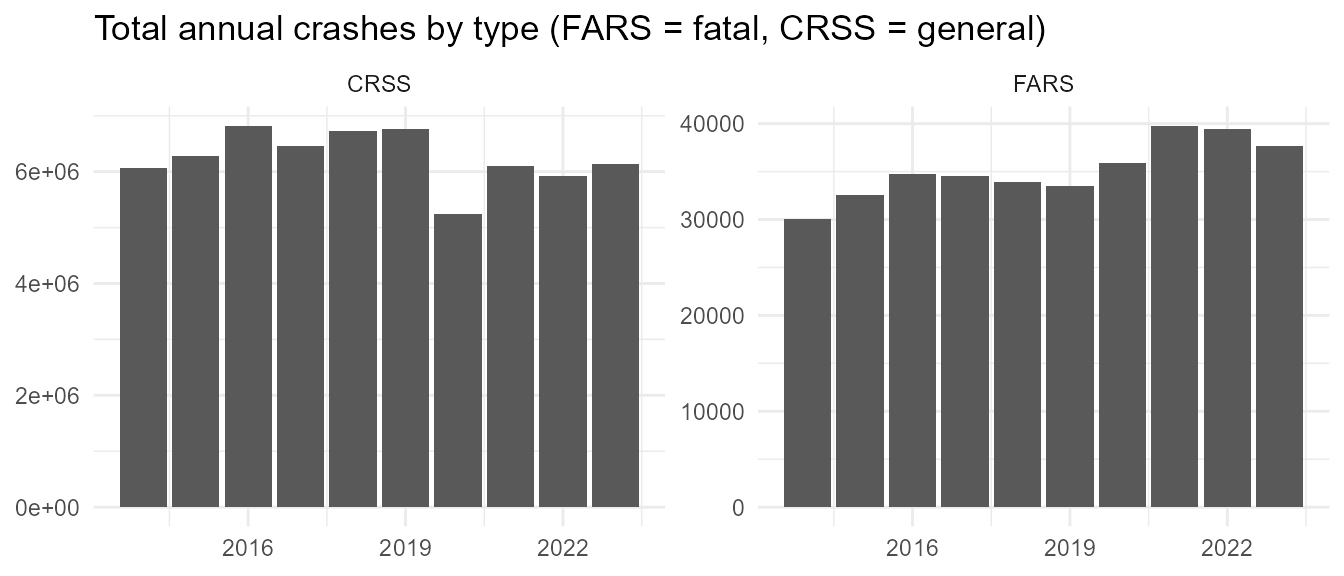
rfars::annual_counts %>%
  filter(source=="FARS", involved != "any") %>%
  ggplot(aes(x=year, y=n)) +
  geom_col() +
  facet_wrap(.~involved, scales = "free_y") +
  labs(title = "Annual fatal crashes by factor involved", subtitle = "Derived from FARS data files", x=NULL, y=NULL) +
  theme_minimal() +
  theme(plot.title.position = "plot")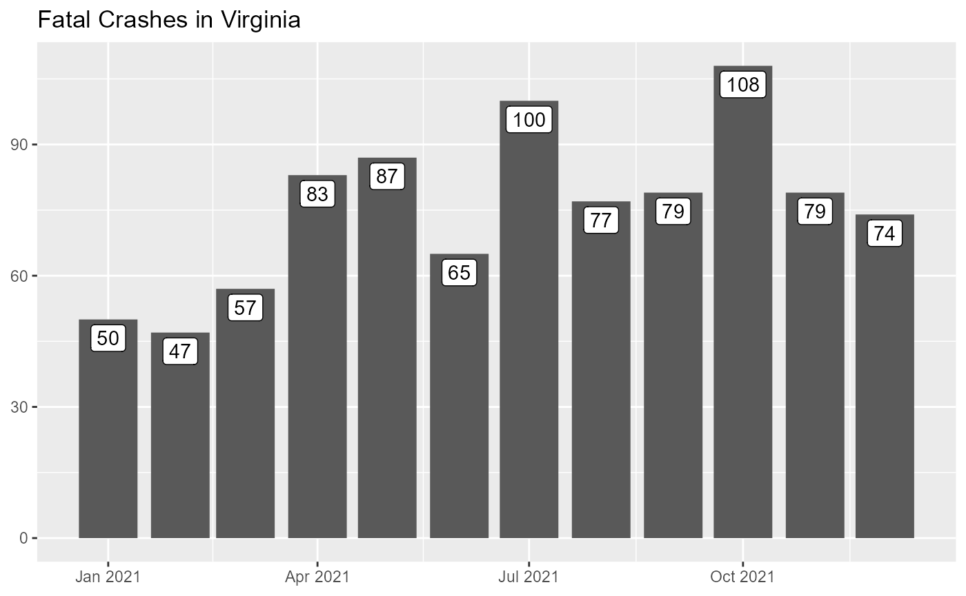
rfars::annual_counts %>%
  filter(source=="CRSS", involved != "any") %>%
  ggplot(aes(x=year, y=n)) +
  geom_col() +
  facet_wrap(.~involved, scales = "free_y") +
  labs(title = "Annual crashes of all severity levels by factor involved", subtitle = "Derived from CRSS data files", x=NULL, y=NULL) +
  theme_minimal() +
  theme(plot.title.position = "plot")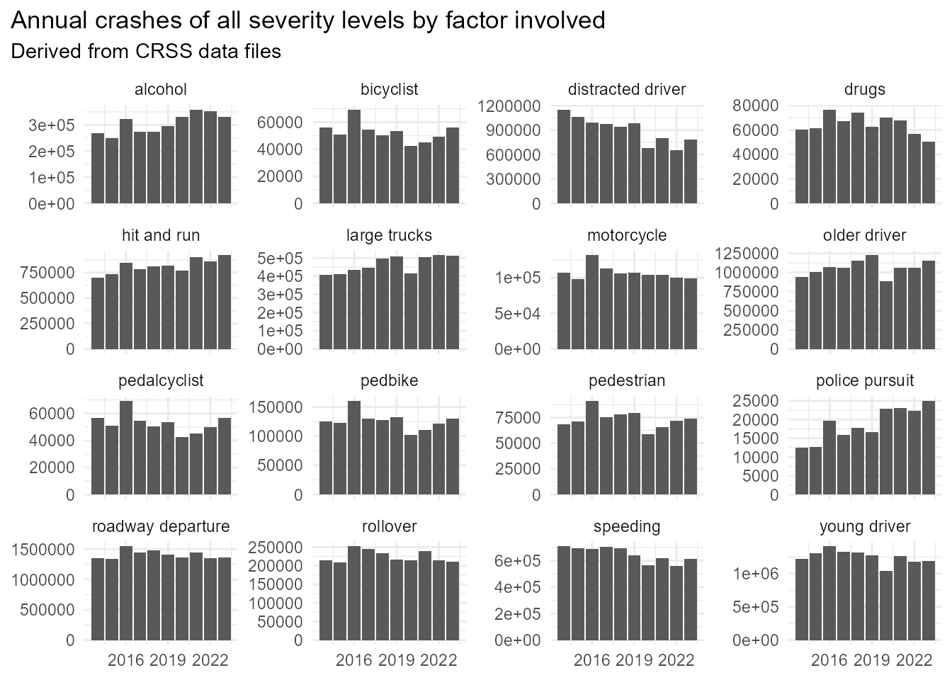
Generating Custom Counts
We can use get_fars() and then counts() to generate a variety of custom counts. Below we pull the latest 5 years of data for Virginia:
myFARS <- get_fars(years = 2019:2023, proceed = T, states = "VA")Then we can use counts() to get the monthly number of
crashes in Virginia:
my_counts <- counts(
  df = myFARS,
  where = list(states = "VA"),
  what = "crashes",
  interval = c("year", "month")
  )
This returns the following dataframe:
knitr::kable(my_counts, format = "html")| year | month | what | states | region | urb | who | involved | n |
|---|---|---|---|---|---|---|---|---|
| 2020 | Jan | crashes | VA | all | all | all | any | 64 |
| 2020 | Feb | crashes | VA | all | all | all | any | 57 |
| 2020 | Mar | crashes | VA | all | all | all | any | 57 |
| 2020 | Apr | crashes | VA | all | all | all | any | 47 |
| 2020 | May | crashes | VA | all | all | all | any | 55 |
| 2020 | Jun | crashes | VA | all | all | all | any | 74 |
| 2020 | Jul | crashes | VA | all | all | all | any | 79 |
| 2020 | Aug | crashes | VA | all | all | all | any | 78 |
| 2020 | Sep | crashes | VA | all | all | all | any | 80 |
| 2020 | Oct | crashes | VA | all | all | all | any | 72 |
| 2020 | Nov | crashes | VA | all | all | all | any | 56 |
| 2020 | Dec | crashes | VA | all | all | all | any | 77 |
| 2021 | Jan | crashes | VA | all | all | all | any | 50 |
| 2021 | Feb | crashes | VA | all | all | all | any | 47 |
| 2021 | Mar | crashes | VA | all | all | all | any | 57 |
| 2021 | Apr | crashes | VA | all | all | all | any | 83 |
| 2021 | May | crashes | VA | all | all | all | any | 87 |
| 2021 | Jun | crashes | VA | all | all | all | any | 65 |
| 2021 | Jul | crashes | VA | all | all | all | any | 100 |
| 2021 | Aug | crashes | VA | all | all | all | any | 77 |
| 2021 | Sep | crashes | VA | all | all | all | any | 79 |
| 2021 | Oct | crashes | VA | all | all | all | any | 108 |
| 2021 | Nov | crashes | VA | all | all | all | any | 79 |
| 2021 | Dec | crashes | VA | all | all | all | any | 74 |
| 2022 | Jan | crashes | VA | all | all | all | any | 62 |
| 2022 | Feb | crashes | VA | all | all | all | any | 84 |
| 2022 | Mar | crashes | VA | all | all | all | any | 63 |
| 2022 | Apr | crashes | VA | all | all | all | any | 58 |
| 2022 | May | crashes | VA | all | all | all | any | 84 |
| 2022 | Jun | crashes | VA | all | all | all | any | 84 |
| 2022 | Jul | crashes | VA | all | all | all | any | 82 |
| 2022 | Aug | crashes | VA | all | all | all | any | 87 |
| 2022 | Sep | crashes | VA | all | all | all | any | 93 |
| 2022 | Oct | crashes | VA | all | all | all | any | 99 |
| 2022 | Nov | crashes | VA | all | all | all | any | 85 |
| 2022 | Dec | crashes | VA | all | all | all | any | 63 |
| 2023 | Jan | crashes | VA | all | all | all | any | 78 |
| 2023 | Feb | crashes | VA | all | all | all | any | 49 |
| 2023 | Mar | crashes | VA | all | all | all | any | 60 |
| 2023 | Apr | crashes | VA | all | all | all | any | 75 |
| 2023 | May | crashes | VA | all | all | all | any | 77 |
| 2023 | Jun | crashes | VA | all | all | all | any | 72 |
| 2023 | Jul | crashes | VA | all | all | all | any | 69 |
| 2023 | Aug | crashes | VA | all | all | all | any | 92 |
| 2023 | Sep | crashes | VA | all | all | all | any | 85 |
| 2023 | Oct | crashes | VA | all | all | all | any | 69 |
| 2023 | Nov | crashes | VA | all | all | all | any | 71 |
| 2023 | Dec | crashes | VA | all | all | all | any | 59 |
| 2024 | Jan | crashes | VA | all | all | all | any | 62 |
| 2024 | Feb | crashes | VA | all | all | all | any | 62 |
| 2024 | Mar | crashes | VA | all | all | all | any | 62 |
| 2024 | Apr | crashes | VA | all | all | all | any | 72 |
| 2024 | May | crashes | VA | all | all | all | any | 89 |
| 2024 | Jun | crashes | VA | all | all | all | any | 83 |
| 2024 | Jul | crashes | VA | all | all | all | any | 68 |
| 2024 | Aug | crashes | VA | all | all | all | any | 84 |
| 2024 | Sep | crashes | VA | all | all | all | any | 80 |
| 2024 | Oct | crashes | VA | all | all | all | any | 80 |
| 2024 | Nov | crashes | VA | all | all | all | any | 66 |
| 2024 | Dec | crashes | VA | all | all | all | any | 59 |
Which we can graph:
my_counts %>%
  mutate_at("year", factor) %>%
  ggplot(aes(x=month, y=n, group=year, color=year, label=scales::comma(n))) +
  geom_line(linewidth = 1.5, alpha=.9) +
  scale_color_brewer() +
  labs(x=NULL, y=NULL, title = "Fatal Crashes in Virginia") +
  theme(plot.title.position = "plot")
my_counts %>%
  mutate(date = lubridate::make_date(year, month)) %>%
  ggplot(aes(x=date, y=n, label=scales::comma(n))) +
  geom_col() +
  labs(x=NULL, y=NULL, title = "Fatal Crashes in Virginia")  +
  theme(plot.title.position = "plot")
We could alternatively count annual fatalities:
counts(
  myFARS,
  where = list(states = "VA"),
  what = "fatalities",
  interval = c("year")
  ) %>%
knitr::kable(format = "html")| year | what | states | region | urb | who | involved | n |
|---|---|---|---|---|---|---|---|
| 2020 | fatalities | VA | all | all | all | any | 850 |
| 2021 | fatalities | VA | all | all | all | any | 973 |
| 2022 | fatalities | VA | all | all | all | any | 1006 |
| 2023 | fatalities | VA | all | all | all | any | 914 |
| 2024 | fatalities | VA | all | all | all | any | 917 |
Or fatalities involving speeding:
counts(
  df = myFARS,
  where = list(states = "VA"),
  what = "fatalities",
  interval = c("year"),
  involved = "speeding"
) %>%
knitr::kable(format = "html")| year | what | states | region | urb | who | involved | n |
|---|---|---|---|---|---|---|---|
| 2020 | fatalities | VA | all | all | all | speeding | 257 |
| 2021 | fatalities | VA | all | all | all | speeding | 337 |
| 2022 | fatalities | VA | all | all | all | speeding | 299 |
| 2023 | fatalities | VA | all | all | all | speeding | 323 |
| 2024 | fatalities | VA | all | all | all | speeding | 285 |
Or fatalities involving speeding in rural areas:
counts(
  myFARS,
  where = list(states = "VA", urb="rural"),
  what = "fatalities",
  interval = c("year"),
  involved = "speeding"
) %>%
knitr::kable(format = "html")| year | what | states | region | urb | who | involved | n |
|---|---|---|---|---|---|---|---|
| 2020 | fatalities | VA | all | rural | all | speeding | 116 |
| 2021 | fatalities | VA | all | rural | all | speeding | 176 |
| 2022 | fatalities | VA | all | rural | all | speeding | 148 |
| 2023 | fatalities | VA | all | rural | all | speeding | 158 |
| 2024 | fatalities | VA | all | rural | all | speeding | 133 |
Or we can use involved = ‘each’ to see all of the problems in one state:
counts(
  df = myFARS,
  where = list(states = "VA"),
  what = "crashes",
  interval = "year",
  involved = "each"
) %>%
  pivot_wider(names_from = "year", values_from = "n") %>%
  arrange(desc(`2023`)) %>%
knitr::kable(format = "html")| what | states | region | urb | who | involved | 2020 | 2021 | 2022 | 2023 | 2024 |
|---|---|---|---|---|---|---|---|---|---|---|
| crashes | VA | all | all | all | roadway departure | 477 | 539 | 507 | 475 | 485 |
| crashes | VA | all | all | all | speeding | 233 | 307 | 276 | 294 | 267 |
| crashes | VA | all | all | all | rollover | 177 | 211 | 316 | 276 | 286 |
| crashes | VA | all | all | all | alcohol | 259 | 267 | 259 | 235 | 256 |
| crashes | VA | all | all | all | older driver | 170 | 215 | 208 | 193 | 217 |
| crashes | VA | all | all | all | pedbike | 117 | 141 | 179 | 143 | 148 |
| crashes | VA | all | all | all | motorcycle | 101 | 117 | 118 | 128 | 120 |
| crashes | VA | all | all | all | pedestrian | 110 | 125 | 168 | 128 | 124 |
| crashes | VA | all | all | all | large trucks | 95 | 109 | 109 | 110 | 110 |
| crashes | VA | all | all | all | young driver | 85 | 108 | 108 | 102 | 98 |
| crashes | VA | all | all | all | distracted driver | 103 | 103 | 82 | 48 | 64 |
| crashes | VA | all | all | all | hit and run | 37 | 34 | 51 | 38 | 35 |
| crashes | VA | all | all | all | drugs | 29 | 32 | 37 | 21 | 30 |
| crashes | VA | all | all | all | police pursuit | 19 | 20 | 11 | 19 | 17 |
| crashes | VA | all | all | all | bicyclist | 7 | 16 | 11 | 15 | 24 |
| crashes | VA | all | all | all | pedalcyclist | 7 | 16 | 11 | 15 | 24 |
Comparing Counts
We can use compare_counts() to quickly produce
comparison graphs. Below we compare speeding-related fatalities in rural
and urban areas:
compare_counts(
  df = myFARS,
  interval = "year",
  involved = "speeding",
  what = "fatalities",
  where = list(states = "VA", urb="rural"),
  where2 = list(states = "VA", urb="urban")
  ) %>%
  ggplot(aes(x=factor(year), y=n, label=scales::comma(n))) +
    geom_col() +
    geom_label(vjust=1.2) +
    facet_wrap(.~urb) +
labs(x=NULL, y=NULL, title = "Speeding-Related Fatalities in Virginia", fill=NULL) 
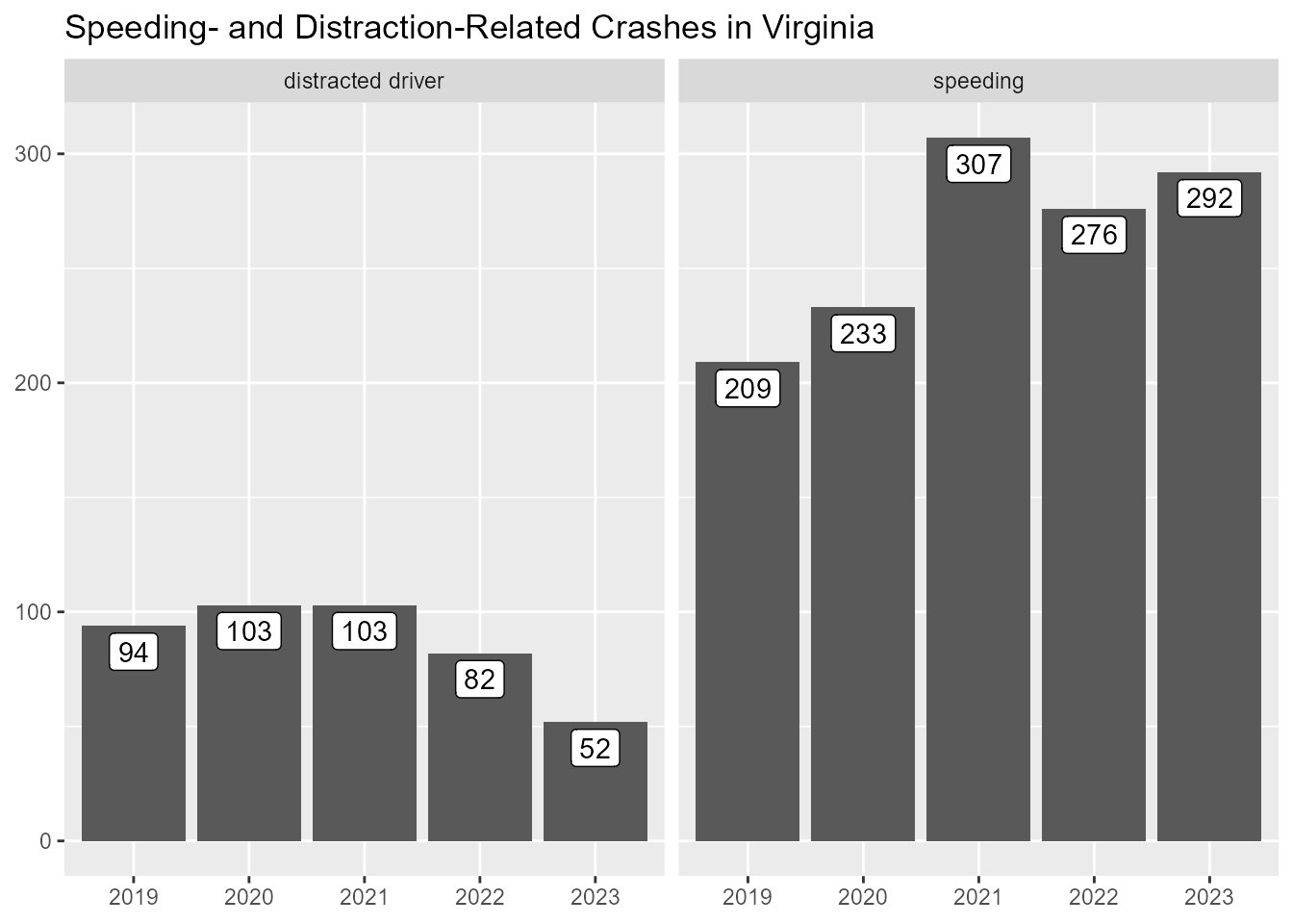
And here we compare speeding-related crashes to those related to distraction:
compare_counts(
  df = myFARS,
  where = list(states = "VA"),
  interval = "year",
  involved = "speeding",
  involved2 = "distracted driver",
  what = "crashes",
  ) %>%
  ggplot(aes(x=factor(year), y=n, label=scales::comma(n))) +
    geom_col() +
    geom_label(vjust=1.2) +
    facet_wrap(.~involved) +
    labs(x=NULL, y=NULL, title = "Speeding- and Distraction-Related Crashes in Virginia", fill=NULL)